Yearly Archives: 2021


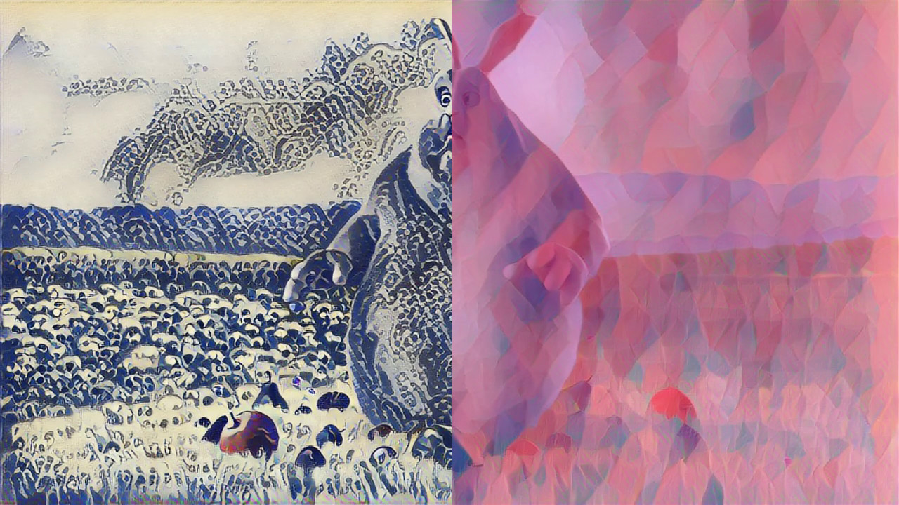
Using Neural Style Transfer on videos

We decided to revisit some old work on Neural Style Transfer and TensorFlow. Using the sample code for Fast Neural Style Transfer from this page https://www.tensorflow.org/tutorials/generative/style_transfer#fast_style_transfer_using_tf-hub and the image stylization model from here https://tfhub.dev/google/magenta/arbitrary-image-stylization-v1-256/2, we created a tool.

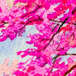
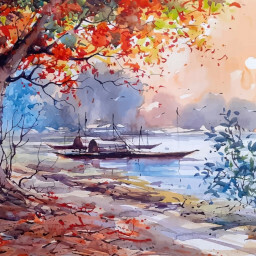
The goal of our venture was to simplify the procedure of changing the style of media. The input could either be an image, a series of images, a video, or a group of videos.

This tool (for which the code is below) comprises a bash script and a python code.
On a high level, it reads all videos from one folder and all styles from another. Then it recreates all those videos with all those styles making new videos out of combinations of the two.

Hardware

Please note that we enabled CUDA and GPU processing on our computer before using the tool. Without them, execution would be prolonged dramatically due to the inability of a general-purpose CPU to make many mathematic operations as fast as the GPU.
To enable CUDA, we followed the steps found in these notes: https://bytefreaks.net/gnulinux/rough-notes-on-how-to-install-cuda-on-an-ubuntu-20-04lts

Software

Conda / Anaconda

We installed and activated anaconda on an Ubuntu 20.04LTS desktop. To do so, we installed the following dependencies from the repositories:

sudo apt-get install libgl1-mesa-glx libegl1-mesa libxrandr2 libxrandr2 libxss1 libxcursor1 libxcomposite1 libasound2 libxi6 libxtst6;

Then, we downloaded the 64-Bit (x86) Installer from (https://www.anaconda.com/products/individual#linux).

Using a terminal, we followed the instructions here (https://docs.anaconda.com/anaconda/install/linux/) and performed the installation.

Python environment and OpenCV for Python

Following the previous step, we used the commands below to create a virtual environment for our code. We needed python version 3.9 (as highlighted here https://www.anaconda.com/products/individual#linux) and the following packages tensorflow matplotlib tensorflow_hub for python.

source ~/anaconda3/bin/activate;
conda create --yes --name FastStyleTransfer python=3.9;
conda activate FastStyleTransfer;
pip install --upgrade pip;
pip install tensorflow matplotlib tensorflow_hub;

faster.py

import matplotlib.pylab as plt
import numpy as np
import tensorflow as tf
import tensorflow_hub as hub

from os import listdir
from os.path import isfile, join

import argparse

print("TF Version: ", tf.__version__)
print("TF Hub version: ", hub.__version__)
print("Eager mode enabled: ", tf.executing_eagerly())
print("GPU available: ", tf.config.list_physical_devices('GPU'))

# Parsing command line arguments while making sure they are mandatory/required
parser = argparse.ArgumentParser()
parser.add_argument(
    "--input",
    type=str,
    required=True,
    help="The directory that contains the input video frames.")
parser.add_argument(
    "--output",
    type=str,
    required=True,
    help="The directory that will contain the output video frames.")
parser.add_argument(
    "--style",
    type=str,
    required=True,
    help="The location of the style frame.")


# Press the green button in the gutter to run the script.
if __name__ == '__main__':
    
    args = parser.parse_args()
    input_path = args.input + '/'
    output_path = args.output + '/'
    # List all files from the input directory. This directory should contain at least one image/video frame.
    onlyfiles = [f for f in listdir(input_path) if isfile(join(input_path, f))]

    # Loading the input style image.
    style_image_path = args.style  # @param {type:"string"}
    style_image = plt.imread(style_image_path)

    # Convert to float32 numpy array, add batch dimension, and normalize to range [0, 1]. Example using numpy:
    style_image = style_image.astype(np.float32)[np.newaxis, ...] / 255.

    # Optionally resize the images. It is recommended that the style image is about
    # 256 pixels (this size was used when training the style transfer network).
    # The content image can be any size.
    style_image = tf.image.resize(style_image, (256, 256))
    
    # Load image stylization module.
    # Enable the following line and disable the next two to load the stylization module from a local folder.
    # hub_module = hub.load('magenta_arbitrary-image-stylization-v1-256_2')
    # Disable the above line and enable these two to load the stylization module from the internet.
    hub_handle = 'https://tfhub.dev/google/magenta/arbitrary-image-stylization-v1-256/2'
    hub_module = hub.load(hub_handle)
 

    for inputfile in onlyfiles:
        content_image_path = input_path + inputfile  # @param {type:"string"}
        content_image = plt.imread(content_image_path)
        # Convert to float32 numpy array, add batch dimension, and normalize to range [0, 1]. Example using numpy:
        content_image = content_image.astype(np.float32)[np.newaxis, ...] / 255.

        # Stylize image.
        outputs = hub_module(tf.constant(content_image), tf.constant(style_image))
        stylized_image = outputs[0]

        # Saving stylized image to disk.
        content_outimage_path = output_path + inputfile  # @param {type:"string"}
        tf.keras.utils.save_img(content_outimage_path, stylized_image[0])


The above code can be invoked as follows:

python3 faster.py --input "$input_frames_folder" --output "$output_frames_folder" --style "$style";

It requires the user to define:

  1. The folder in which all input images should be.
  2. The folder where the user wants the stylized images to be saved in. Please note that the folder needs to be created by the user before the execution.
  3. The path to the image that will be used as input to the neural style transfer.

execute.sh

#!/bin/bash
#source ~/anaconda3/bin/activate;
#conda create --yes --name FastStyleTransfer python=3.9;
#pip install --upgrade pip;
#pip install tensorflow matplotlib tensorflow_hub;
#conda activate FastStyleTransfer;

source ~/anaconda3/bin/activate;
conda activate FastStyleTransfer;

input_videos="./input/videos/*";
input_styles="./input/styles/*";
input_frames="./input/frames";
input_audio="./input/audio";
output_frames="./output/frames";
output_videos="./output/videos";

# Loop on each video in the input folder.
for video in $input_videos;
do
  echo "$video";
  videoname=$(basename "$video");

  # Extract all frames from the video file and save them in a new folder using 8-digit numbers with zero padding in an incremental order.
  input_frames_folder="$input_frames/$videoname";
  mkdir -p "$input_frames_folder";
  ffmpeg -v quiet -i "$video" "$input_frames_folder/%08d.ppm";

  # Extract the audio file from the video to the format of an mp3. We will need this audio later to add it to the final product.
  input_audio_folder="$input_audio/$videoname";
  mkdir -p "$input_audio_folder";

  audio="";
  # Only VP8 or VP9 or AV1 video and Vorbis or Opus audio and WebVTT subtitles are supported for WebM.
  if [[ $videoname == *.webm ]]; then
    audio="$input_audio_folder/$videoname.ogg";
    ffmpeg -v quiet -i "$video" -vn -c:a libvorbis -y "$audio";  
  else
    audio="$input_audio_folder/$videoname.mp3";
    ffmpeg -v quiet -i "$video" -vn -c:a libmp3lame -y "$audio";
  fi

  # Retrieve the frame rate from the input video. We will need it to configure the final video later.
  frame_rate=`ffprobe -v 0 -of csv=p=0 -select_streams v:0 -show_entries stream=r_frame_rate "$video"`;

  # Loop on each image style from the input styles folder.
  for style in $input_styles;
  do
    echo "$style";
    stylename=$(basename "$style");
    output_frames_folder="$output_frames/$videoname/$stylename";
    mkdir -p "$output_frames_folder";

    # Stylize all frames using the input image and write all processed frames to the output folder.
    python3 faster.py --input "$input_frames_folder" --output "$output_frames_folder" --style "$style";

    # Combine all stylized video frames and the exported audio into a new video file.
    output_videos_folder="$output_videos/$videoname/$stylename";
    mkdir -p "$output_videos_folder";
    ffmpeg -v quiet -framerate "$frame_rate" -i "$output_frames_folder/%08d.ppm" -i "$audio" -pix_fmt yuv420p -acodec copy -y "$output_videos_folder/$videoname";
    
    rm -rf "$output_frames_folder";
  done
  rm -rf "$output_frames/$videoname";
  rm -rf "$input_frames_folder";
  rm -rf "$input_audio_folder";
done

The above script does not accept parameters, but you should load the appropriate environment before calling it. For example:

source ~/anaconda3/bin/activate;
conda activate FastStyleTransfer;
./execute.sh;

Please note that this procedure consumes significant space on your hard drive; once you are done with a video, you should probably delete all data from the output folders.


Rough notes on how to install CUDA on an Ubuntu 20.04LTS 1

To anyone coming across this post, please note that Canonical does not officially support CUDA. Not being supported formally means that you could face problems that we did not while setting up our machine.

Recently we wanted to use our GPU to execute various TensorFlow projects. We had to use version 1, specifically version 1.15 of TensorFlow, on one of our attempts. That setup was causing many problems even after version 2 was working perfectly. There must be something different with version 1, and it is not supported correctly anymore. We recommend avoiding using it unless needed.

Finding out what graphics card we have

Before getting started, we executed the following command that gave us the model of our graphics card:

lspci | grep -i nvidia;
$ lspci | grep -i nvidia
01:00.0 VGA compatible controller: NVIDIA Corporation TU104 [GeForce RTX 2080 Rev. A] (rev a1)
01:00.1 Audio device: NVIDIA Corporation TU104 HD Audio Controller (rev a1)
01:00.2 USB controller: NVIDIA Corporation TU104 USB 3.1 Host Controller (rev a1)
01:00.3 Serial bus controller [0c80]: NVIDIA Corporation TU104 USB Type-C UCSI Controller (rev a1)

Installing dependencies and NVidia repositories

Then we proceeded to install the headers of our Linux kernel, the repositories of NVidia, and finally install CUDA using apt-get.

sudo apt-get install linux-headers-$(uname -r);
wget https://developer.download.nvidia.com/compute/cuda/repos/ubuntu2004/x86_64/cuda-ubuntu2004.pin;
sudo mv cuda-ubuntu2004.pin /etc/apt/preferences.d/cuda-repository-pin-600;
sudo apt-key adv --fetch-keys https://developer.download.nvidia.com/compute/cuda/repos/ubuntu2004/x86_64/7fa2af80.pub;
sudo add-apt-repository "deb https://developer.download.nvidia.com/compute/cuda/repos/ubuntu2004/x86_64/ /";
sudo apt-get update;
sudo apt-get -y install cuda;
sudo apt-get install nvidia-gds;

After this step, we rebooted the computer to load the NVidia graphics driver.


Playing with shadow(s)

The passwords are stored in a digital fingerprint using salt (salted hash) in the Linux system through the crypt function. You can find relevant information about the implementation in Ubuntu at http://manpages.ubuntu.com/manpages/bionic/man3/crypt.3.html (how to call this function, what the arguments are etc.) Assume that you have managed to access a secret shadow file of an Ubuntu Linux system (see the shadow file contents below). The system has two users, bob and alice.

alice:$6$.s6xaWmE$m9KjrSJ1dgZ20M5IhEyXORNV.KZwBk5hp1XZ0mpOyTe.dGET.EdMCFgPimkeM7nWEW4wejMoVV.40Cg6w9XJ..:17470:0:99999:7:::
bob:$6$aACNZdTj$GYrSPRP.ieCiUfmFFRwKwEByU2rdSdfP4gCij1asUgT.dpmmu3NIDLAAde5cfvNtacI9JUGQUgrBciUWAUWNY1:17470:0:99999:7:::

Tasks

Based on the information you will obtain from the above link, which hash function did the system use to generate the salted hashed passwords?

From the documentation, we get the following information:

The glibc2 version of this function supports additional encryption algorithms.

If salt is a character string starting with the characters "$id$"  followed  by  a  string
optionally terminated by "$", then the result has the form:

      $id$salt$encrypted

id  identifies  the encryption method used instead of DES and this then determines how the
rest of the password string is interpreted.  The following values of id are supported:

      ID  | Method
      ─────────────────────────────────────────────────────────
      1   | MD5
      2a  | Blowfish (not in mainline glibc; added in some
          | Linux distributions)
      5   | SHA-256 (since glibc 2.7)
      6   | SHA-512 (since glibc 2.7)

We can see in both lines of our shadow file, that between the first and second colon (:) the hashed value is following the format described above. This means that the id of the function used is between the first and second dollar sign ($) and that value is in both cases the value 6. From this result, we know that SHA-512 was used.

Which salt was used for bob and which for alice?

The salt that was used for bob is .s6xaWmE and the salt for alice aACNZdTj. We get this data on each line, between the second dollar sign ($) and the third.

From the shadow file, can you see for sure if alice and bob have chosen different passwords? Explain your answer.

Since the system used different salt while hashing each password, we cannot infer any information regarding the similarity of the passwords of bob and alice.

Your goal is to discover the passwords of these two users. To do this, you have some information about the personal life of bob and alice:

For the bob user, you know that he is now starting to learn how to use computers. He is unaware of security risks and has probably chosen an easy password (one that many users generally select).

For alice, you know some of her personal information: her phone number is 6955345671, her license plate is ZKA4221, and she likes the Rolling Stones. Alice has only a limited knowledge of security. She knows it is suitable for a password to combine letters with numbers and have several characters. Still, she does not fully understand how to choose a secure password.

Please describe the actions you will take to guess their passwords, doing your tests on the shadow file. For bob, use lists of common passwords, while for alice, use the above personal information.

To get the password of bob, we used a simple approach using John the Ripper (lovely tool by the way). As seen in the following commands, we installed John the Ripper and using the default settings we asked John to crack any passwords in our shadow file.

sudo snap install john-the-ripper;
john shadow ;

IIn seconds, John the Ripper produced the password for the user bob, which was 1234567890. John the Ripper was so quick that it felt like magic! Unfortunately (or fortunately, depending on the context), John the Ripper cannot do magic… The reason it was so fast, in this case, is because the default settings for John the Ripper instruct the tool to try many simple passwords first using wordlist files. We already knew that bob was using one of those passwords, so it made the selection of options trivial.

At this stage, it would appear that the password for alice was harder to guess, and John the Ripper did not produce a result after we let it execute for a few minutes. Something that is worth mentioning about the case of bob is the following; We could have asked John the Ripper to try and crack the password using all alphanumeric characters only ([a-z][A-Z][0-9]). It would have taken longer, but it could work since we knew from Human Intelligence (HumInt) that bob is using fairly simple passwords.

Below is the raw output of the console for the case of cracking the password of bob. Please note that we used ctrl+c to kill the execution as we did not expect John the Ripper to get the password for alice as well.

$ john shadow 
Created directory: /home/bob/snap/john-the-ripper/459/.john
Warning: detected hash type "sha512crypt", but the string is also recognized as "HMAC-SHA256"
Use the "--format=HMAC-SHA256" option to force loading these as that type instead
Warning: detected hash type "sha512crypt", but the string is also recognized as "sha512crypt-opencl"
Use the "--format=sha512crypt-opencl" option to force loading these as that type instead
Using default input encoding: UTF-8
Loaded 2 password hashes with 2 different salts (sha512crypt, crypt(3) $6$ [SHA512 256/256 AVX2 4x])
Cost 1 (iteration count) is 5000 for all loaded hashes
Will run 12 OpenMP threads
Proceeding with single, rules:Single
Press 'q' or Ctrl-C to abort, almost any other key for status
Warning: Only 46 candidates buffered for the current salt, minimum 48 needed for performance.
Warning: Only 45 candidates buffered for the current salt, minimum 48 needed for performance.
Almost done: Processing the remaining buffered candidate passwords, if any.
Warning: Only 43 candidates buffered for the current salt, minimum 48 needed for performance.
Warning: Only 33 candidates buffered for the current salt, minimum 48 needed for performance.
Proceeding with wordlist:/snap/john-the-ripper/current/run/password.lst, rules:Wordlist
1234567890       (bob)
Proceeding with incremental:ASCII

To tackle the case of alice, we had to improvise a bit. First of all, we made a text file that on each line it contained the personal information that Human Intelligence gathered for us about alice. To ensure that John the Ripper would have more material to work with, we also did some variations to some data, like splitting the license plate into two tokens. The file (keywords.lst) looked like so:

6955345671
ZKΑ4221
Rolling Stones
alice
zka4221
zka
4221
Stones
Rolling

Then, we used hashcat to create a new list that would combine the previous tokens making more complex passwords. We had this hint from the Human Intelligence analysis, so it was an easy choice to make. The new and amazing list (advanced.lst) that we created had the following data in it:

sudo apt-get install hashcat;
#Type in the contents of the list above
nano keywords.lst;
#Not sure why it requires sudo
sudo hashcat -a 1 --stdout keywords.lst keywords.lst > advanced.lst;
69553456716955345671
6955345671ZKΑ4221
6955345671Rolling Stones
6955345671alice
6955345671zka4221
6955345671zka
69553456714221
6955345671Stones
6955345671Rolling
ZKΑ42216955345671
ZKΑ4221ZKΑ4221
ZKΑ4221Rolling Stones
ZKΑ4221alice
ZKΑ4221zka4221
ZKΑ4221zka
ZKΑ42214221
ZKΑ4221Stones
ZKΑ4221Rolling
Rolling Stones6955345671
Rolling StonesZKΑ4221
Rolling StonesRolling Stones
Rolling Stonesalice
Rolling Stoneszka4221
Rolling Stoneszka
Rolling Stones4221
Rolling StonesStones
Rolling StonesRolling
alice6955345671
aliceZKΑ4221
aliceRolling Stones
alicealice
alicezka4221
alicezka
alice4221
aliceStones
aliceRolling
zka42216955345671
zka4221ZKΑ4221
zka4221Rolling Stones
zka4221alice
zka4221zka4221
zka4221zka
zka42214221
zka4221Stones
zka4221Rolling
zka6955345671
zkaZKΑ4221
zkaRolling Stones
zkaalice
zkazka4221
zkazka
zka4221
zkaStones
zkaRolling
42216955345671
4221ZKΑ4221
4221Rolling Stones
4221alice
4221zka4221
4221zka
42214221
4221Stones
4221Rolling
Stones6955345671
StonesZKΑ4221
StonesRolling Stones
Stonesalice
Stoneszka4221
Stoneszka
Stones4221
StonesStones
StonesRolling
Rolling6955345671
RollingZKΑ4221
RollingRolling Stones
Rollingalice
Rollingzka4221
Rollingzka
Rolling4221
RollingStones
RollingRolling

To use the above custom wordlist on the shadow file, we issued the following command to John the Ripper:

john --wordlist=advanced.lst --rules shadow;

A few moments later, John the Ripper produced the following output indicating that the password for alice was rollingstones4221.

$ john --wordlist=advanced.lst --rules shadow
Warning: detected hash type "sha512crypt", but the string is also recognized as "HMAC-SHA256"
Use the "--format=HMAC-SHA256" option to force loading these as that type instead
Warning: detected hash type "sha512crypt", but the string is also recognized as "sha512crypt-opencl"
Use the "--format=sha512crypt-opencl" option to force loading these as that type instead
Using default input encoding: UTF-8
Loaded 2 password hashes with 2 different salts (sha512crypt, crypt(3) $6$ [SHA512 256/256 AVX2 4x])
Remaining 1 password hash
Cost 1 (iteration count) is 5000 for all loaded hashes
Will run 12 OpenMP threads
Press 'q' or Ctrl-C to abort, almost any other key for status
rollingstones4221 (alice)
1g 0:00:00:00 DONE (2021-11-26 17:09) 3.846g/s 3765p/s 3765c/s 3765C/s 69553456716955345671..Rollingstonesing
Use the "--show" option to display all of the cracked passwords reliably
Session completed

Bonus Material

Finding previously cracked passwords

A tip for people that are new to John the Ripper. In case you forgot to write down all passwords that were produced; you can issue the following command that will show you all the passwords that John the Ripper knows for the specific input file:

john --show shadow;
$ john --show shadow
alice:rollingstones4221:17470:0:99999:7:::
bob:1234567890:17470:0:99999:7:::

2 password hashes cracked, 0 left

Trying to crack a shadow file using Python

In case you would like to use programming and manually crack the shadow file, there are ways.
Using the Python language and the crypt package, we can write a simple program. The program will accept the salt and the unencrypted input text and produce the hashed output. It would be the same result; as a result, a Linux machine would make while creating its shadow file.

import crypt
from hmac import compare_digest as compare_hash

crypt.crypt("1234567890", "$6$aACNZdTj$")
#It would produce the following, which is the salted hash for the password of bob
#'$6$aACNZdTj$GYrSPRP.ieCiUfmFFRwKwEByU2rdSdfP4gCij1asUgT.dpmmu3NIDLAAde5cfvNtacI9JUGQUgrBciUWAUWNY1'

Notes on how to get HarpyTM running on an Ubuntu 20.04LTS GNU/Linux

Easy Setup – Slow Execution by using the CPUs only

Getting CUDA support in OpenCV for Python can be tricky as you will need to make several changes to your PC. On many occasions, it can fail if you are not comfortable troubleshooting the procedure. For this reason, we are presenting an alternative solution that is easy to implement and should work on most machines. The problem with this solution is that it will ignore your GPU and utilize your CPUs only. This means that executions will most probably be slower than the GPU-enabled one.

Conda / Anaconda

First of all, we installed and activated anaconda on an Ubuntu 20.04LTS desktop. To do so, we installed the following dependencies from the repositories:

sudo apt-get install libgl1-mesa-glx libegl1-mesa libxrandr2 libxrandr2 libxss1 libxcursor1 libxcomposite1 libasound2 libxi6 libxtst6;

Then, we downloaded the 64-Bit (x86) Installer from (https://www.anaconda.com/products/individual#linux).

Using a terminal, we followed the instructions here (https://docs.anaconda.com/anaconda/install/linux/) and performed the installation.

Python environment and OpenCV for Python

Following the previous step, we used the commands below to create a virtual environment for our code. We needed python version 3.9 (as highlighted here https://www.anaconda.com/products/individual#linux) and OpenCV for python.

source ~/anaconda3/bin/activate;
conda create --yes --name HarpyTM python=3.9;
conda activate HarpyTM;
pip install numpy scipy scikit-learn opencv-python==4.5.1.48;

Please note that we needed to limit the package for opencv-python to 4.5.1.48 because we were getting the following error on newer versions:

python3 Monitoring.py 
./data/DJI_0406_cut.MP4
[INFO] setting preferable backend and target to CUDA...
Traceback (most recent call last):
  File "/home/bob/Traffic/HarpyTM/Monitoring.py", line 51, in <module>
    detectNet = detector(weights, config, conf_thresh=conf_thresh, netsize=cfg_size, nms_thresh=nms_thresh, gpu=use_gpu, classes_file=classes_file)
  File "/home/bob/Traffic/HarpyTM/src/detector.py", line 24, in __init__
    self.layers = [ln[i[0] - 1] for i in self.net.getUnconnectedOutLayers()]
  File "/home/bob/Traffic/HarpyTM/src/detector.py", line 24, in <listcomp>
    self.layers = [ln[i[0] - 1] for i in self.net.getUnconnectedOutLayers()]
IndexError: invalid index to scalar variable.

Usage

git clone https://github.com/rafcy/HarpyTM;
cd HarpyTM/;
# We manually create the following folders and set their priviledges as we were  getting errors when they were autogenerated by the code of HarpyTM.
mkdir -p results/Detections/videos;
chmod 777 results/Detections/videos;

After successfully cloning the project, we modified the config.ini to meet our needs, specifically, we changed all paths to be inside the folder of HarpyTM and used the full resolution for the test video:

[Video]
video_filename 		= ./data/DJI_0406_cut.MP4
resize 			= True
image_width 		= 1920
image_height 		= 1080
display_video		= False
display_width 		= 1920
display_height 		= 1080


[Export]
save_video_results	= True
video_export_path 	= ./results/Detections/videos/
csv_path 		= ./results/
export			= True
display_track		= True

[Detector]
#darknet
darknet_config 		= ./data/Configs/vehicles_ty3.cfg
darknet_weights 	= ./data/Configs/vehicles_ty3.weights
classes_file 		= ./data/Configs/vehicles.names
cfg_size_width		= 608
cfg_size_height		= 608
iou_thresh 		= 0.3
conf_thresh 		= 0.3
nms_thresh 		= 0.4
use_gpu 		= True 

[Tracker]
flight_height 		= 150
sensor_height 		= 0.455
sensor_width		= 0.617
focal_length		= 0.567
reset_boxes_frames	= 40
calc_velocity_n		= 25
draw_tracks		= True
export_data		= True

Finally, we were able to execute the code as follows:

python3 Monitoring.py;

After the execution was done, we found in the folder ./results/Detections/videos/ the video showing the bounding boxes etc. The resulting video was uploaded here: