In the world of spreadsheet applications, LibreOffice Calc stands out as a versatile and powerful tool for managing data. It offers a wide array of features that can help you organize, analyze, and make sense of your data. One of these features, often underutilized, is the Subtotals functionality. In this blog post, we’ll explore how to use the Subtotals functionality in the Data menu of LibreOffice Calc to count how many times each item is repeated in a dataset. This is particularly useful when working with large datasets or lists, as it allows you to create summary reports without the need for complex formulas or manual counting.
Preparing Your Data
Start by opening LibreOffice Calc and loading the dataset you want to analyze. Ensure that your data is organized in columns and that each item you want to count is in a separate column. For example, if you have a list of products, each product name should be in its own column.
Sorting Your Data
To use the Subtotals functionality effectively, your data needs to be sorted by the column containing the items you want to count. To sort your data:
Select the entire dataset by clicking and dragging your mouse.
Go to the “Data” menu, and then click on “Sort.”
Sort Data
In the “Sort Criteria” dialog box, select the column containing the items you want to count.
Choose the sorting order (ascending or descending), and click “OK.”
Your data is now sorted and ready for subtotal analysis.
Using the Subtotals Functionality
With your data sorted, you can now use the Subtotals functionality:
Select the entire dataset again.
Go to the “Data” menu and click on “Subtotals.”
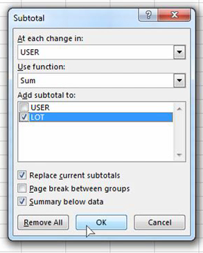
Subtotals
In the “Subtotals” dialog box, you’ll see options for grouping and summarizing your data. By default, it may suggest using the first column for grouping, which is what you want in most cases.
Subtotals Dialog
In the “Function” dropdown, choose the type of summary you want, which is “Count” in this case.
Make sure that the “Replace current subtotals” option is selected.
Click “OK.”
LibreOffice Calc will now calculate the subtotal counts for each item in your dataset and insert them into your spreadsheet. It will also group items together and provide an outline to help you navigate the summary.
Subtotals Result
The Subtotals functionality creates a summary of your data by grouping items and counting them. You can expand and collapse these groups using the outlined symbols to the left of the spreadsheet. This allows you to view the summary data in a more organized manner.
The Subtotals functionality in LibreOffice Calc is a powerful tool for analyzing data and generating summary reports. Whether you’re working with product lists, customer data, or any other dataset, Subtotals can help you count how many times each item is repeated without the need for complex formulas or manual counting. By following the steps outlined in this blog post, you can harness the full potential of LibreOffice Calc and make your data analysis tasks more efficient and accurate. Give it a try, and you’ll be amazed at how Subtotals can streamline your data analysis workflow.
The following examples allow you to convert hexadecimal values of the format 0xYYYYYY to decimal using a spreadsheet editor like Calc or Excel.
The following codes will remove the first two characters (the value 0x) of the cell B2 and then convert the result to decimal using the HEX2DEC function.
Using the RIGHT function
In this example, we used the RIGHT function with the num_chars parameter to be equal to the number of characters in the cell minus 2. This used to delete the 0x value from the HEX column by removing the first two characters of the cell.
To get the number of characters in the cell we use the LEN function on the cell of interest.
=HEX2DEC(RIGHT(B2,LEN(B2)-2))
Using the SUBSTITUTE function
In the following example we used the SUBSTITUTE function to automatically find the 0x prefix of the HEX value and delete it by replacing it with an empty string.
=HEX2DEC(SUBSTITUTE(B2,"0x",""))
Using the REPLACE function
The last example uses the REPLACE function. Starting from the character in position 1 in the cell, it replaces the sub-string of size 2 with the empty string and thus deleting the prefix. Please note that this function is not zero-based so the first character is at position 1 and not at position 0.
=HEX2DEC(REPLACE(B2,1,2,""))
Functions Legend:
RIGHT(text,[num_chars]) – RIGHT returns the last character or characters in a text string, based on the number of characters you specify in the variable num_chars. RIGHT always counts each character, whether single-byte or double-byte, as 1, no matter what the default language setting is.
LEN(text) – LEN returns the number of characters in a text string. Again, LEN always counts each character, whether single-byte or double-byte, as 1, no matter what the default language setting is.
HEX2DEC(number) – HEX2DEC converts a hexadecimal number to decimal.
SUBSTITUTE(text, old_text, new_text, [instance_num]) – Substitutes new_text for old_text in a text string. You can use SUBSTITUTE when you want to replace specific text in a text string.
REPLACE(old_text, start_num, num_chars, new_text) – REPLACE replaces part of a text string, based on the number of characters you specify, with a different text string. Use REPLACE when you want to replace any text that occurs in a specific location in a text string. REPLACE always counts each character, whether single-byte or double-byte, as 1, no matter what the default language setting is.
In the following video we demonstrate how to randomize the rows of an Excel sheet.
Methodology:
We created a new column next to the data we want to randomize their order, then we typed in the first cell the following formula =rand(). =rand() will generate a random value between 0 and 1.
After that we applied the same formula to the entire column.
To apply the formula to the whole column we used a very simple method: we double-clicked on the bottom right hand corner of the cell .
Later, we sorted our date using the column of random values.
Finally, we deleted the new column.
Alternative way to copy the formula to the entire column:
Including the cell with the formula, select the cells in the new column that you want the new formula applied to (all the rows you want to be randomized) and the press Ctrl+D.