csv


Analyzing Data with Python: Counting how many times each value in a CSV occurs

Data analysis is an essential aspect of many fields, from business and research to sports and education. Python, with its versatile libraries, is a popular choice for data analysis tasks. In this blog post, we’ll explore a Python script that reads data from a CSV file and counts the occurrences of each value in 3 columns. The script can be a valuable tool for gaining insights into educational information datasets.

#!/bin/python

import csv

# Create empty dictionaries
d_university = dict()
d_country = dict()
d_region = dict()

with open('XtremeScores.csv') as f:
    reader = csv.reader(f, delimiter=',', quoting=csv.QUOTE_NONE)
    # Loop through each line of the file
    for line in reader:
        word = line[6]
        # Check if the word is already in dictionary
        if word in d_region:
            # Increment count of word by 1
            d_region[word] = d_region[word] + 1
        else:
            # Add the word to dictionary with count 1
            d_region[word] = 1

        word = line[5]
        # Check if the word is already in dictionary
        if word in d_country:
            # Increment count of word by 1
            d_country[word] = d_country[word] + 1
        else:
            # Add the word to dictionary with count 1
            d_country[word] = 1

        word = line[4]
        # Check if the word is already in dictionary
        if word in d_university:
            # Increment count of word by 1
            d_university[word] = d_university[word] + 1
        else:
            # Add the word to dictionary with count 1
            d_university[word] = 1

sorted_university = sorted(d_university.items(), key=lambda x:x[1], reverse=True)
print(sorted_university[:10])
sorted_country = sorted(d_country.items(), key=lambda x:x[1], reverse=True)
print(sorted_country[:10])
sorted_region = sorted(d_region.items(), key=lambda x:x[1], reverse=True)
print(sorted_region[:10])

Let’s break down the code step by step:

#!/bin/python

import csv

The script starts by importing the csv module, which is essential for handling comma-separated value (CSV) files.

# Create empty dictionaries
d_university = dict()
d_country = dict()
d_region = dict()

Three empty dictionaries, d_university, d_country, and d_region, are created. These dictionaries will be used to store the counts of universities, countries, and regions, respectively.

with open('XtremeScores.csv') as f:
    reader = csv.reader(f, delimiter=',', quoting=csv.QUOTE_NONE)

The script opens a CSV file named ‘XtremeScores.csv’ using a with statement. The csv.reader object is used to read the contents of the file. We specify that the delimiter is a comma (,), and we don’t want to perform any special quoting.

    # Loop through each line of the file
    for line in reader:

A for loop iterates through each line in the CSV file. The variable line contains the data for each row in the file.

        word = line[6]

The code extracts the word at index 6 (zero-based index) from the current line. In this context, it typically represents a region.

        # Check if the word is already in the dictionary
        if word in d_region:
            # Increment count of word by 1
            d_region[word] = d_region[word] + 1
        else:
            # Add the word to the dictionary with count 1
            d_region[word] = 1

The code checks if the extracted word (representing a region) is already present in the d_region dictionary. If it is, it increments the count by 1. If not, it adds the word to the dictionary with a count of 1. This process counts the occurrences of each region in the dataset.

The code repeats the same process for words representing countries (at index 5) and universities (at index 4), using the d_country and d_university dictionaries, respectively.

sorted_university = sorted(d_university.items(), key=lambda x:x[1], reverse=True)
print(sorted_university[:10])

After counting the universities, the code sorts them in descending order of frequency and prints the top 10 universities based on their occurrence.

sorted_country = sorted(d_country.items(), key=lambda x:x[1], reverse=True)
print(sorted_country[:10])

Similarly, it does the same for countries and prints the top 10 countries.

sorted_region = sorted(d_region.items(), key=lambda x:x[1], reverse=True)
print(sorted_region[:10])

Finally, it sorts and prints the top 10 regions based on their occurrence.

In summary, this Python script provides a simple but effective way to analyze data in a CSV file, specifically counting universities, countries, and regions. It leverages dictionaries to maintain counts and uses the csv module for reading data from the file. This can be a useful starting point for more advanced data analysis tasks and visualization in Python.


Python script to parse the GAM / Google Workspace CSV that contains all members of all groups

This script will parse the data generated by GAM and create an XLSX out of them.

Each sheet will be named by the group, containing all the emails of that group, including the sub-groups.

# This script will parse the data generated by GAM and create an XLSX out of them.
# Each sheet will be named by the group and it will contain all the emails of that group, including the sub-groups.

# Using sys to get command line arguments for the input file
import sys
# Using CSV to parse the input CSV file that GAM (GAMADV-XTD3) created after using the following command:
# gam print group-members > emails.2022.csv;
# Source: https://bytefreaks.net/google/rough-notes-on-using-gam-to-print-all-members-of-all-groups-in-google-workspace
import csv
# Using pandas to create an XLSX file with multiple sheets
import pandas as pd

# Creating an empty dictionary.
dictionary = {}

# Opening the CSV file that is the first command line argument
with open(sys.argv[1], newline='') as csvfile:
    reader = csv.reader(csvfile, delimiter=',', quotechar='"')
    # For each row, we are getting only the first column which is the group and the last which is the email
    for row in reader:
        dictionary.setdefault(row[0], []).append(row[5])

# Create a Pandas Excel writer using XlsxWriter as the engine.
writer = pd.ExcelWriter(sys.argv[1]+'.xlsx', engine='xlsxwriter')

# Iterating in Sorted Order
for key in sorted(dictionary):
    # Create a Pandas dataframes to add the data.
    df = pd.DataFrame({'Members': dictionary[key]})
    # Write each dataframe to a different worksheet.
    # To avoid the following exception:
    # xlsxwriter.exceptions.InvalidWorksheetName: Excel worksheet name '[email protected]' must be <= 31 chars.
    # We are truncating the domain from the group.
    group = key.split("@")[0]
    # In case the name is still to big, we truncate it further and append an ellipsis to indicate the extra truncation
    sheet = (group[:29] + '..') if len(group) > 31 else group
    # We are also removing the header and index of the data frame
    df.to_excel(writer, sheet_name=sheet, header=False, index=False)

# Close the Pandas Excel writer and output the Excel file.
writer.close()

[GnuPlot] Create a plot with Date Time on X axis

Download here : [download id=”1309″]

The following script, will read the ‘data.csv’ file and create a plot with the data.
The input file (data.csv) should have two columns: the first one is a date/time string and the second is a number.
e.g

2016-01-19 13:12:38,2
2016-01-19 13:12:38,1
2016-01-19 13:12:38,0
2016-01-19 13:12:40,0
2016-01-19 13:12:41,0
2016-01-19 13:12:47,0

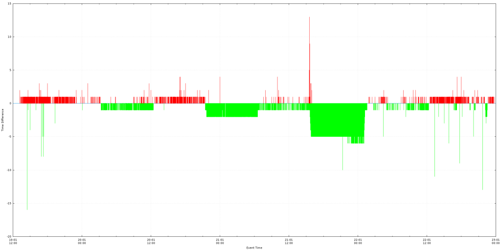
The chart will have on the X axis the date/time and on the Y axis the value of the second column.
All values under the 0 axis will be green and all values above it will be red.

Example output:

data.csv

Execution example: gnuplot -e "filename='data.csv'; width=2000; height=1000;" timeDifference.plot

#Setting output to be a PNG file of size 'width'x'height'
#'width' and 'height' are set from the command line. e.g gnuplot -e "filename='server_1.csv'; width=10000; height=500;" timeDifference.plot
#Setting the font of all text to be 'Verdana' size 8
set terminal pngcairo size width,height enhanced font 'Verdana,8'
#Setting the output filename to be the same as the input filename with the .png extension appended to it.
set output filename.'.png'

#We set the file separator to be the comma, this way we inform the engine that we will be processing a CSV file
set datafile separator ","

#Informing the engine that the X axis of our plot will be date/time data type
set xdata time
#We define how the date/time input must be parsed. In this example we expect the input to be like '2016-01-19 14:25:00'
set timefmt '%Y-%m-%d %H:%M:%S'

#We set the output format that will be shown on the X axis. Here we expect to show '19-01 New Line 14:25"
set format x "%d-%m\n%H:%M"
#Set the X axis label
set xlabel "Event Time"
#Set the Y axis label
set ylabel "Time Difference" 

#Enabling the Grid, this way major tick lines will be visible on the chart
set grid

#As we expect to have negative values as well, we make the zero Y axis line is thicker and has a different style from the rest so that it will be easier to spot
set xzeroaxis linetype 3 linewidth 1.5

#Creating a style for the lines that will be used in the plot. Type = 1, Color = green, Width = 1
set style line 1 linetype 1 linecolor rgb "green" linewidth 1.000
#Creating a style for the lines that will be used in the plot. Type = 1, Color = red, Width = 1
set style line 2 linetype 1 linecolor rgb "red" linewidth 1.000

#Actual plot command
#It directs the engine to plot the file that is in the filename variable, use the first and second column and use vertical columns with the styles we described above
#First line, We will plot only values that are greater or equal to 0, the rest we give 1/0 which is an invalid number and will not be plotted
#Second line, We will plot only values that are strictly less than 0, the rest we give 1/0 which is an invalid number and will not be plotted
plot filename using 1:($2 <= 0?$2:1/0) with impulses ls 1 notitle,\
filename using 1:($2 <= 0?1/0:$2) with impulses ls 2 notitle