
1. INTRODUCTION
Page 2
Machine learning algorithms must be trained using a large set of known data and then tested using another independent set before it is used on unknown data.
The result of running a machine learning algorithm can be expressed as a
function y(x) which takes a new x as input and that generates an output vector y, encoded in the same way as the target vectors. The precise form of the function y(x) is determined during the training phase, also known as the learning phase, on the basis of the training data. Once the model is trained it can then determine the identity of new elements, which are said to comprise a test set. The ability to categorize correctly new examples that differ from those used for training is known as generalization. In practical applications, the variability of the input vectors will be such that the training data can comprise only a tiny fraction of all possible input vectors, and so generalization is a central goal in pattern recognition.
The pre-processing stage is sometimes also called feature extraction. Note that new test data must be pre-processed using the same steps as the training data. The aim is to find useful features that are fast to compute, and yet that also preserve useful discriminatory information. Care must be taken during pre-processing because often information is discarded, and if this information is important to the solution of the problem then the overall accuracy of the system can suffer.
Page 3
Applications in which the training data comprises examples of the input vectors along with their corresponding target vectors are known as supervised learning problems. Cases such as the digit recognition example, in which the aim is to assign each input vector to one of a finite number of discrete categories, are called classification problems. If the desired output consists of one or more continuous variables, then the task is called regression. An example of a regression problem would be the prediction of the yield in a chemical manufacturing process in which the inputs consist of the concentrations of reactants, the temperature, and the pressure.
In other pattern recognition problems, the training data consists of a set of input
vectors x without any corresponding target values. The goal in such unsupervised learning problems may be to discover groups of similar examples within the data, where it is called clustering, or to determine the distribution of data within the input space, known as density estimation, or to project the data from a high-dimensional space down to two or three dimensions for the purpose of visualization.
Finally, the technique of reinforcement learning (Sutton and Barto, 1998) is concerned with the problem of finding suitable actions to take in a given situation in order to maximize a reward. Here the learning algorithm is not given examples of optimal outputs, in contrast to supervised learning, but must instead discover them by a process of trial and error. Typically there is a sequence of states and actions in which the learning algorithm is interacting with its environment. In many cases, the current action not only affects the immediate reward but also has an impact on the reward at all subsequent time steps.
The reward must then be attributed appropriately to all of the moves that led to it, even though some moves will have been good ones and others less so. This is an example of a credit assignment problem. A general feature of reinforcement learning is the trade-off between exploration, in which the system tries out new kinds of actions to see how effective they are, and exploitation, in which
the system makes use of actions that are known to yield a high reward.
1.1 Example: Polynomial Curve Fitting
Page 5
We fit the data using a polynomial function of the form:
[latex]y(x, w) = w_{0}x^{0} + w_{1}x^{1} + w_{2}x^{2} + . . . + w_{M}x^{M} = \sum_{j =0}^{M}w_{j}x^{j}[/latex]
where M is the order of the polynomial.
The values of the coefficients will be determined by fitting the polynomial to the
training data. This can be done by minimizing an error function that measures the misfit between the function y(x, w), for any given value of w, and the training set data points.
Our error function: Sum of the squares of the errors between the predictions [latex]y(x_{n} , w)[/latex] for each data point [latex]x_n[/latex] and the corresponding target values [latex]t_n[/latex].
[latex]E(w) = \frac{1}{2}\sum_{n=1}^{N}\{y(x_{n},w) – t_{n}\}^2[/latex]
Much higher order polynomial can cause Over-Fitting : the fitted curve oscillates wildly and gives a very poor representation of the function.
We can obtain some quantitative insight into the dependence of the generalization performance on M by considering a separate test set comprising 100 data points generated using exactly the same procedure used to generate the training set points but with new choices for the random noise values included in the target values.
Root Mean Square: [latex]E_{RMS} = \sqrt{2E(w*)/N}[/latex]
The division by N allows us to compare different sizes of data sets on an equal footing, and the square root ensures that [latex]E_{RMS}[/latex] is measured on the same scale (and in the same units) as the target variable t.
OTHER
To study
Curve Fitting
Additional Terms
Legend:
- TP = True Positive
- TN = True Negative
- FP = False Positive
- FN = False Negative
[latex]correct\ rate (accuracy) = \frac{TP + TN}{TP + TN + FP + FN}[/latex]
[latex]sensitivity = \frac{TP}{TP + FN}[/latex]
[latex]specificity = \frac{TN}{TN + FP}[/latex]
Receiver Operating Characteristic
In statistics, a receiver operating characteristic (ROC), or ROC curve, is a graphical plot that illustrates the performance of a binary classifier system as its discrimination threshold is varied. The curve is created by plotting the true positive rate (sensitivity) against the false positive rate (1 – specificity) at various threshold settings.
— From https://en.wikipedia.org/wiki/Receiver_operating_characteristic
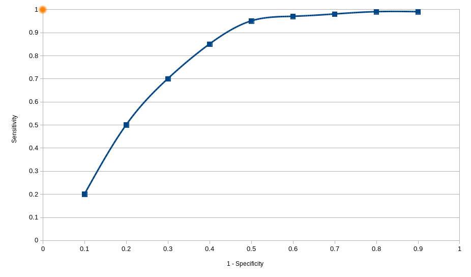 Assuming we have a system where changing its configuration we get the above results, we would pick the configuration that has the smallest Euclidean Distance from the perfect configuration. The perfect configuration can be found at point (0,1) where both Specificity and Sensitivity are both equal to one.
Chapters to ignore
Non – Parametric
This post is also available in: Αγγλικα

